
This post will show you how to add Text Boxes to a chart.
Excel has text boxes for the Title, horizontal axis and the vertical axis. Sometimes we need to make side comments, such as "Good job" or "Watch this" in other locations on the chart. We do this by adding text boxes.
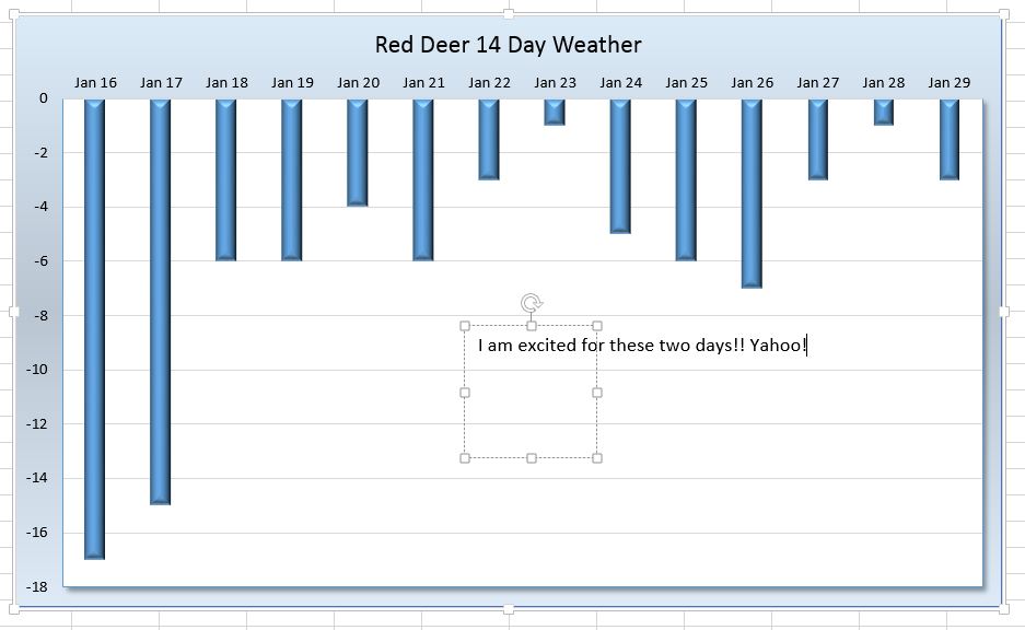
I created the following chart using the weather temperature forecast for the next 14 days.
 1. I want to add a text box in the middle of the chart to express how excited I am for the two warm days. [Jan 23 & 28th]
2. Select the chart that you want to make changes to.
The ribbon now has two new tabs at the end.


5. Move your mouse onto the chart. Your mouse icon is an upside down lowercase letter t.
6. Click where you want the text box to be. Don't stress. You can move it later if it is not exactly correct.

7. Type in what you would like to say. Don't worry if the text goes outside the box. See below.
We will size and arrange the box after all the text is inside.


Excel has text boxes for the Title, horizontal axis and the vertical axis. Sometimes we need to make side comments, such as "Good job" or "Watch this" in other locations on the chart. We do this by adding text boxes.
I created the following chart using the weather temperature forecast for the next 14 days.

2. Select the chart that you want to make changes to.
The ribbon now has two new tabs at the end.
Insert Text Box
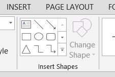
3. Click the Format Tab
4. Click the Text Box icon in the Insert Shapes section of the Format Tab.
6. Click where you want the text box to be. Don't stress. You can move it later if it is not exactly correct.

We will size and arrange the box after all the text is inside.
Size the text box
8. Click in the bottom right-hand corner of the text box. You mouse icon becomes a double arrow on a 45-degree angle.
9. In this example, I dragged the mouse to the right and up so that the box appears around the text as shown in the figure below.

10. Click somewhere else to deselect the text box.
If you would like to format the text, click on the text again and the box around it will appear so you may edit it. Use the Font section of the HOME tab to make changes to the text.
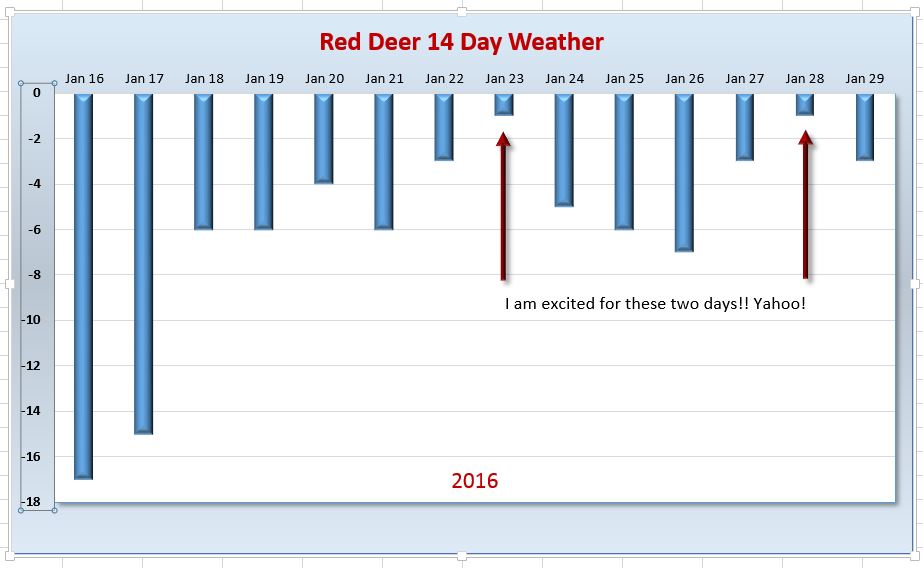
I inserted arrows as well.
I inserted one arrow.
Changed the colour and added some formatting, then copied it and moved the second arrow into another place.
Arrows are also in the Insert Shapes section of the Format Tab.
No comments:
Post a Comment